**DirectX Raytracing, Tutorial 14**
**Swapping out a Lambertian BRDF for a GGX BRDF model**
In [Tutorial 12](../Tutor12/tutorial12.md.html), we showed how to do recursive bounces for path tracing using
a diffuse Lambertain material model. This tutorial explores how to swap out a Lambertian material model for
a more complex model, the [GGX model](https://www.cs.cornell.edu/~srm/publications/EGSR07-btdf.pdf) commonly
used today in film and games. Additionally, we extend the one-bounce global illumination with an arbitrary number
of bounces.
Changes to the C++ Code
=================================================================================
The C++ code barely changes in this tutorial, other than changing the pass names. Inside *`GGXGlobalIllumination.cpp`*,
we ask for a few additional fields from our G-buffer in the `GGXGlobalIlluminationPass::initialize()` method, including the
`MaterialSpecRough` and `Emissive` fields, which include properties needed to render specular materials and those that
emit light directly. This means we can render scenes with no light sources (but materials marked "emissive" will act
as lights).
Additionally, the method `GGXGlobalIlluminationPass::execute()` passes a few additional parameters to our shader,
including a maximum ray depth (`gMaxDepth`) and our additional G-buffer textures.
New Microfacet Functions in the HLSL Code
=================================================================================
A new file in the shader data direction is `microfacentBRDFUtils.hlsli`, which include a number of utility functions
for rendering a GGX material. The form of the GGX BRDF is: `D * G * F / (4 * NdotL * NdotV)`. This form was introduced
by [Cook and Torrance](https://dl.acm.org/citation.cfm?id=357293) (also available [here](http://inst.cs.berkeley.edu/~cs294-13/fa09/lectures/cookpaper.pdf))
and is widely used across many [microfacet BRDF models](http://www.pbr-book.org/3ed-2018/Reflection_Models/Microfacet_Models.html)
used today.
A microfacet BRDF model assumes the surface is made up of a large number of very tiny planar facets that are all perfectly
reflective (i.e., they reflect along the mirror direction). In rough, diffuse surfaces these facets are oriented almost
uniformly randomly so light is reflected evenly around the hemisphere. On glossy surfaces, these facets are much more
likely to lie flat along the geometry. The `D` term is the microfacet distribution, which controls the probability an
incoming ray sees a facet of a particular orientation.
We use a standard form of the GGX normal distribution for D
(e.g., math taken from [here](http://blog.selfshadow.com/publications/s2012-shading-course/hoffman/s2012_pbs_physics_math_notes.pdf)):
~~~~~~~~~~~~~~~~~~~~C
float ggxNormalDistribution( float NdotH, float roughness )
{
float a2 = roughness * roughness;
float d = ((NdotH * a2 - NdotH) * NdotH + 1);
return a2 / (d * d * M_PI);
}
~~~~~~~~~~~~~~~~~~~~
Note: When building path tracers, it is important to maintain numerical robustness to avoid NaNs and Infs. In some
circumstances, the last line in the `ggxNormalDistribution()` function may cause a divide by zero, so you may wish to clamp.
The `G` term in the Cook-Torrance BRDF model represents geometric masking of the microfacets. I.e., facets of various
orientations will not always be visible; they may get occluded by other tiny facets. The model for geometric masking we
use is from [Schlick's BRDF model](https://onlinelibrary.wiley.com/doi/abs/10.1111/1467-8659.1330233)
(or [direct PDF](http://www.cs.virginia.edu/~jdl/bib/appearance/analytic%20models/schlick94b.pdf)). Usually other masking
terms are used with GGX (see [Naty Hoffman's SIGGRAPH Notes](http://blog.selfshadow.com/publications/s2012-shading-course/hoffman/s2012_pbs_physics_math_notes.pdf)),
but this model plugs in robustly without a lot of code massaging, which makes the tutorial code simpler to understand. This
formulation for the Schlick approximation comes from Karas' SIGGRAPH 2013 notes from the Physically Based Shading course:
~~~~~~~~~~~~~~~~~~~~C
float schlickMaskingTerm(float NdotL, float NdotV, float roughness)
{
// Karis notes they use alpha / 2 (or roughness^2 / 2)
float k = roughness*roughness / 2;
// Compute G(v) and G(l). These equations directly from Schlick 1994
// (Though note, Schlick's notation is cryptic and confusing.)
float g_v = NdotV / (NdotV*(1 - k) + k);
float g_l = NdotL / (NdotL*(1 - k) + k);
return g_v * g_l;
}
~~~~~~~~~~~~~~~~~~~~
Finally, the `F` term in the Cook-Torrance model is the [Fresnel term](https://en.wikipedia.org/wiki/Fresnel_equations),
which describes how materials become more reflective when seen from a grazing angle. Rarely do renderers implement the
full Fresnel equations, which account for the wave nature of light. Since most real-time renderers assume [geometric optics](https://en.wikipedia.org/wiki/Geometrical_optics),
we can ignore wave effects, and most renderers use [Schlick's approximation](https://en.wikipedia.org/wiki/Schlick%27s_approximation),
which comes from the same paper references above:
~~~~~~~~~~~~~~~~~~~~C
float3 schlickFresnel(float3 f0, float lDotH)
{
return f0 + (float3(1.0f, 1.0f, 1.0f) - f0) * pow(1.0f - lDotH, 5.0f);
}
~~~~~~~~~~~~~~~~~~~~
Finally, in addition to the three functions representing `D`, `G`, and `F`, the `microfacetBRDFUtils.hlsli` also includes the
function `getGGXMicrofacet()` which gets a random microfacet orientation (i.e., a facet normal) that follows the distribution
described by the function `ggxNormalDistribution()`. This allows us to randomly choose what direction a ray bounces when it
leaves a specular surface:
~~~~~~~~~~~~~~~~~~~~~C
// When using this function to sample, the probability density is:
// pdf = D * NdotH / (4 * HdotV)
float3 getGGXMicrofacet(inout uint randSeed, float roughness, float3 hitNorm)
{
// Get our uniform random numbers
float2 randVal = float2(nextRand(randSeed), nextRand(randSeed));
// Get an orthonormal basis from the normal
float3 B = getPerpendicularVector(hitNorm);
float3 T = cross(B, hitNorm);
// GGX NDF sampling
float a2 = roughness * roughness;
float cosThetaH = sqrt(max(0.0f, (1.0-randVal.x)/((a2-1.0)*randVal.x+1) ));
float sinThetaH = sqrt(max(0.0f, 1.0f - cosThetaH * cosThetaH));
float phiH = randVal.y * M_PI * 2.0f;
// Get our GGX NDF sample (i.e., the half vector)
return T * (sinThetaH * cos(phiH)) +
B * (sinThetaH * sin(phiH)) +
hitNorm * cosThetaH;
}
~~~~~~~~~~~~~~~~~~~~~
Shading a Surface Point
=================================================================================
When shading a point on a surface, we need to invoke these microfacet BRDF functions. To reduce the chance of error, we
combine these into a function and call this function from multiple locations. In particular, inside the ray
generation shader `ggxGlobalIllumination.rt.hlsl`, shading looks as follows:
~~~~~~~~~~~~~~~~~~~~~C
// Add any emissive color from primary rays
shadeColor = gEmitMult * pixelEmissive.rgb;
// Do explicit direct lighting to a random light in the scene
if (gDoDirectGI)
shadeColor += ggxDirect(randSeed, worldPos.xyz, worldNorm.xyz, V,
difMatlColor.rgb, specMatlColor.rgb, roughness);
// Do indirect lighting for global illumination
if (gDoIndirectGI && (gMaxDepth > 0))
shadeColor += ggxIndirect(randSeed, worldPos.xyz, worldNorm.xyz, V,
difMatlColor.rgb, specMatlColor.rgb, roughness, 0);
~~~~~~~~~~~~~~~~~~~~~
Basically, the color at any hitpoint is: the color a surface emits, plus any light directly visible from light sources, plus
light that bounces in via additional bounces along the path.
When we fire indirect rays (see `indirectRay.hlsli`), we shade the closest hit using a similar process:
~~~~~~~~~~~~~~~~~~~~~~C
[shader("closesthit")]
void IndirectClosestHit(inout IndirectRayPayload rayData,
BuiltInTriangleIntersectionAttributes attribs)
{
// Run a helper functions to extract Falcor scene data for shading
ShadingData shadeData = getHitShadingData( attribs, WorldRayOrigin() );
// Add emissive color
rayData.color = gEmitMult * shadeData.emissive.rgb;
// Do direct illumination at this hit location
if (gDoDirectGI)
{
rayData.color += ggxDirect(rayData.rndSeed, shadeData.posW,
shadeData.N, shadeData.V, shadeData.diffuse, shadeData.specular,
shadeData.roughness);
}
// Do indirect illumination (if we haven't traversed too far)
if (rayData.rayDepth < gMaxDepth)
{
rayData.color += ggxIndirect(rayData.rndSeed, shadeData.posW,
shadeData.N, shadeData.V, shadeData.diffuse, shadeData.specular,
shadeData.roughness, rayData.rayDepth);
}
}
~~~~~~~~~~~~~~~~~~~~~~
Direct Lighting Using a GGX Model
=================================================================================
Direct lighting using a GGX model looks very similar to the direct lighting using
Lambertian from [Tutorial 12](../Tutor12/tutorial12.md.html). In particutlar,
we start by picing a random light, extracting it's information from the Falcor
scene representation, and tracing a shadow ray to determine if it is visible.
Note that with many BRDFs, our GGX model consists of a specular lobe and a diffuse lobe. The math for
the diffuse lobe is identical to that in Tutorial 12, we're just adding a new specular lobe to the diffuse term.
If visible, we perform shading using the GGX model (i.e., `D * G * F / (4* NdotL * NdotV)`).
In this case, numerical robustness is improved significantly by cancelling `NdotL` terms in
the GGX lobe to avoid potential divide-by-zero when light hits geometry at a grazing angle. I left
in these cancelled `NdotL` terms in comments to make the math clear.
~~~~~~~~~~~~~~~~~~~~C
float3 ggxDirect(inout uint rndSeed, float3 hit, float3 N, float3 V,
float3 dif, float3 spec, float rough)
{
// Pick a random light from our scene to shoot a shadow ray towards
int lightToSample = min( int(nextRand(rndSeed) * gLightsCount),
gLightsCount - 1 );
// Query the scene to find info about the randomly selected light
float distToLight;
float3 lightIntensity;
float3 L;
getLightData(lightToSample, hit, L, lightIntensity, distToLight);
// Compute our lambertion term (N dot L)
float NdotL = saturate(dot(N, L));
// Shoot our shadow ray to our randomly selected light
float shadowMult = float(gLightsCount) *
shadowRayVisibility(hit, L, gMinT, distToLight);
// Compute half vectors and additional dot products for GGX
float3 H = normalize(V + L);
float NdotH = saturate(dot(N, H));
float LdotH = saturate(dot(L, H));
float NdotV = saturate(dot(N, V));
// Evaluate terms for our GGX BRDF model
float D = ggxNormalDistribution(NdotH, rough);
float G = ggxSchlickMaskingTerm(NdotL, NdotV, rough);
float3 F = schlickFresnel(spec, LdotH);
// Evaluate the Cook-Torrance Microfacet BRDF model
// Cancel NdotL here to avoid catastrophic numerical precision issues.
float3 ggxTerm = D*G*F / (4 * NdotV /* * NdotL */);
// Compute our final color (combining diffuse lobe plus specular GGX lobe)
return shadowMult * lightIntensity * ( /* NdotL * */ ggxTerm +
NdotL * dif / M_PI);
}
~~~~~~~~~~~~~~~~~~~~
Indirect Lighting Using a GGX Model
=================================================================================
Bouncing an indirect ray is somewhat more complex. Since we have both a diffuse lobe and a specular
lobe, we need to sample them somewhat differently; the cosine sampling used for lambertian shading
doesn't have particularly good characteristics for GGX. One way would shoot two rays: one in the diffuse
lobe and one in the specular lobe. But this gets costly, and they converge at different rates.
Instead, we randomly pick whether to shoot an indirect diffuse or indirect glossy ray (see `ggxIndirect()`):
~~~~~~~~~~~~~~~~C
// We have to decide whether we sample our diffuse or specular/ggx lobe.
float probDiffuse = probabilityToSampleDiffuse(dif, spec);
float chooseDiffuse = (nextRand(rndSeed) < probDiffuse);
~~~~~~~~~~~~~~~~
In this case, we choose specular or diffuse based on their diffuse and specular albedos, though this isn't
a particularly well thought out or principaled approach:
~~~~~~~~~~~~~~~~C
float probabilityToSampleDiffuse(float3 difColor, float3 specColor)
{
float lumDiffuse = max(0.01f, luminance(difColor.rgb));
float lumSpecular = max(0.01f, luminance(specColor.rgb));
return lumDiffuse / (lumDiffuse + lumSpecular);
}
~~~~~~~~~~~~~~~~
Going back to `ggxIndirect()`, if we sample our diffuse lobe, the indirect ray looks almost identical to that
from [Tutorial 12](../Tutor12/tutorial12.md.html). We shoot a cosine-distributed ray, return the color,
and divide by the probability of selecting this ray.
~~~~~~~~~~~~~~~~C
if (chooseDiffuse)
{
// Shoot a randomly selected cosine-sampled diffuse ray.
float3 L = getCosHemisphereSample(rndSeed, N);
float3 bounceColor = shootIndirectRay(hit, L, gMinT, 0, rndSeed, rayDepth);
// Accumulate the color: (NdotL * incomingLight * dif / pi)
// Probability of sampling this ray: (NdotL / pi) * probDiffuse
return bounceColor * dif / probDiffuse;
}
~~~~~~~~~~~~~~~~
If we choose to sample the GGX lobe, the behavior is fundamentally identical even though the code is more complex:
select a random ray, shoot it and return a color, and divide by the probability of selecting this ray. The key
is that when we sample according to `getGGXMicrofacet()` our probability density for our rays is different
(and described by `D * NdotH / (4 * LdotH)`).
~~~~~~~~~~~~~~~~C
// Otherwise we randomly selected to sample our GGX lobe
else
{
// Randomly sample the NDF to get a microfacet in our BRDF
float3 H = getGGXMicrofacet(rndSeed, rough, N);
// Compute outgoing direction based on this (perfectly reflective) facet
float3 L = normalize(2.f * dot(V, H) * H - V);
// Compute our color by tracing a ray in this direction
float3 bounceColor = shootIndirectRay(hit, L, gMinT, 0, rndSeed, rayDepth);
// Compute some dot products needed for shading
float NdotL = saturate(dot(N, L));
float NdotH = saturate(dot(N, H));
float LdotH = saturate(dot(L, H));
// Evaluate our BRDF using a microfacet BRDF model
float D = ggxNormalDistribution(NdotH, rough);
float G = ggxSchlickMaskingTerm(NdotL, NdotV, rough);
float3 F = schlickFresnel(spec, LdotH);
float3 ggxTerm = D * G * F / (4 * NdotL * NdotV);
// What's the probability of sampling vector H from getGGXMicrofacet()?
float ggxProb = D * NdotH / (4 * LdotH);
// Accumulate color: ggx-BRDF * lightIn * NdotL / probability-of-sampling
// -> Note: Should really cancel and simplify the math above
return NdotL * bounceColor * ggxTerm / (ggxProb * (1.0f - probDiffuse));
}
~~~~~~~~~~~~~~~~
What Does it Look Like?
===============================================================================
That covers the important points of this tutorial. When running, you get the following result:
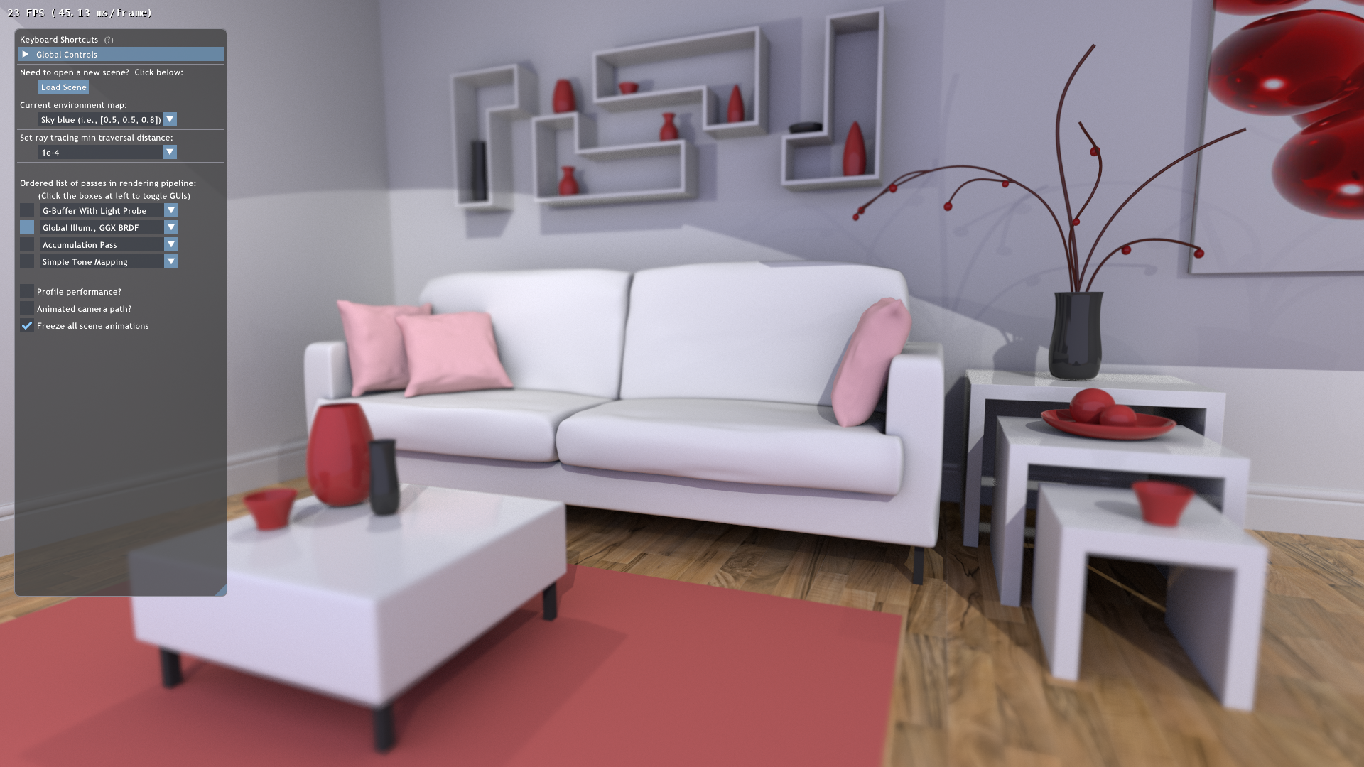
With this tutorial, you can run Falcor's using a fairly feature-rich path tracer, even if the sampling
is extremely naive. Moving forward, which is left as an exercise to the reader, you can add better
importance sampling, multiple importance sampling, and using next-event estimation for better explicit
direct lighting. Additionally, we haven't handled refractive materials in this set of tutorials,
though as described in Pete Shirley's [Ray Tracing in One Weekend](https://github.com/petershirley/raytracinginoneweekend),
this is fairly straightforward to add.